high mix manufacturing


Harmonic, Inc.

 DEHART CONSULTING, INC., working hand-in-hand with our factory personnel, redesigned our manufacturing areas and material flows to enable a 250% growth in output with only a 70% increase in floor space. Additionally, the changes were documented, implemented, and provided a clear path for future expansion. 


Mike Yost, Vice President, Operations Harmonic, Inc.


Using Standard Labor/Machine Processing Hours
     In the case where all units in a WO are processed as a discrete set, the Flow Time of a WO in a WC is equal to the Standard Process Hours of the WO.

Adjusting for Serial Lot-Splitting
    In the case where there are multiple, and serial, operations within the WC and the WO is split into multiple batches within the operations, the Standard Process Hours is adjusted to reflect the actual Flow Time.  The situation is illustrated in the following figure for a WO of twenty units with three serial operations within the WC and a batch size of five.

serial lot splitting

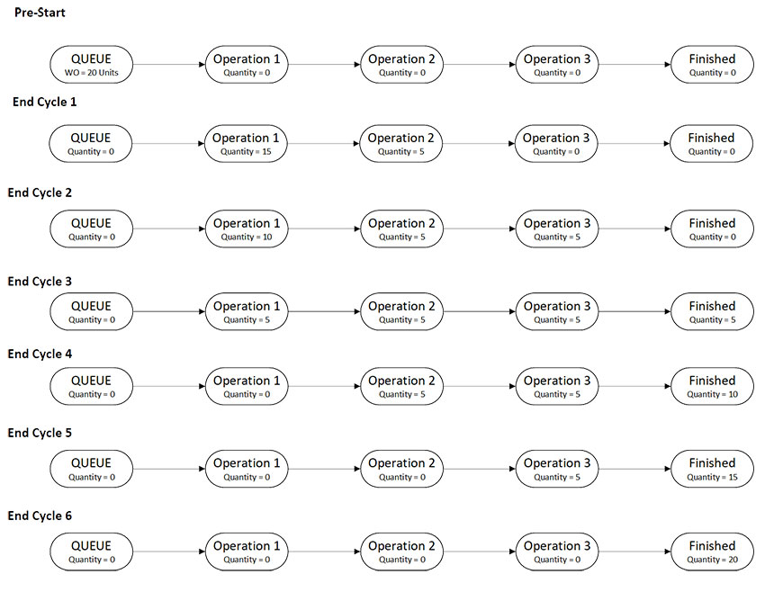
    For example, a WO with a Standard Hour per Unit (HPU) of one-hour per operation, or three hours total.  The total Standard Hours for this WO is then sixty hours and, if worked on at a single operation, or even moved from operation-to-operation as a single batch, the Flow Time would indeed be sixty hours.  But when the WO is split into smaller batches, and moved from operation-to-operation as each batch is completed, the simultaneity of work activities will tend to compress the Flow Time.  In the example shown above, each batch would move every five hours, the operation cycle-time or takt time, and the WO would complete queue-to-finished after six cycles, or just thirty hours, 50% of the Standard Hours.  Thus, this Flow Time compression effect should be taken into account in the case of sequential batch-processing.  

    The Flow Time of a WO at a WC is an essential component in this disclosure and is embodied in the previously defined variables tWO1, n-1, tR,N, QN, YN, tR,N-1, and tQ,N-1.  To account for the serial-lot-split case illustrated above, an adjustment to convert Standard Hours to Flow Time is applied to these factors on a WO-WC basis.

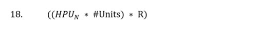
    In particular, an adjustment is made and it should take the form of a ratio that can be applied to the Standard Process Hours:

equation 3

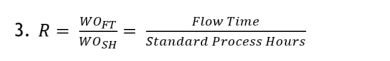
This ratio will vary at each WC and for each WO based on batch sizes and numbers of operations and is derived as follows:

    The batch size that is processed through the WC for a WO is the quantity of units within the WO divided by the number of batches into which the WO is to be split, BN.

equation 4

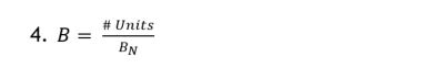
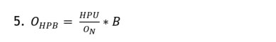
In a balanced line, the operation cycle-time for each batch is equal, or nearly equal, for all operations and is the HPU for the WO divided by the number of operations, ON, (to give HPU per operation) multiplied by the batch size. Expressing this in terms of a single batch gives:

equation 5

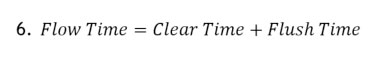
The Flow Time, WOFT, is the amount of elapsed time between the first batch starting at the first operation and the last batch finishing at the last operation. This can be broken up into two segments. The first segment is the amount of time that it takes to complete all batches through the first operation, which is the “Clear Time”.  The second segment is the amount of time it takes to complete all batches through the rest of the operations, which is the “Flush Time.”  Flow Time is the sum of these two times:

 equation 6

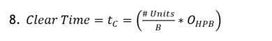
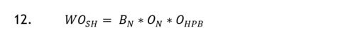
Clear Time can be computed as the number of batches times the OHPB.

equation 7

Or

equation 8

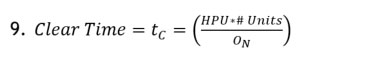
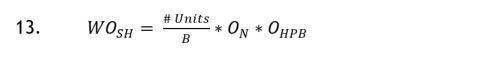
Alternatively, this variation is used to calculate QN, tR, N, and tR, N-1 in the pull-test algorithm, by substituting equation 5 for the value of OHPB, and Clear Time can be expressed as:

equation 9

 The Flush Time is the time required for the last Batch to get though the rest of the Operations, not counting the first one since it was counted in the Clear Time, or

equation 10

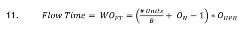
Adding the two segments together yields the following:

equation 11

The denominator of the ratio R from equation 3, Total Standard Hours (WOSH), will equal the sum of the amount of time that each batch spends at each operation. This can be expressed as a simple multiplication of the number of batches by the number of Operations and by the Operational hours per batch.

equation 12

Or

equation 13

Now that both the Total Standard Hours and Flow Time are represented in terms of Quantity, Number of Operations, and Batch Size the ratio between the two values can be calculated. This ratio is the conversion factor for converting Standard Hours into Flow time from equation 3. Substituting the results from equations 11 and 13 into equation 3:

equation 14

equation 15

equation 16

equation 17

An example:

# Units=20; ON=3; B=5; HPU=3

Using equation 4, these values yield 4 for the number of batches that will flow through the WC:

example 1

Using equation 12, this gives a value of Total Standard Hours of 60:

example 2

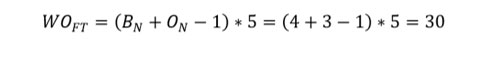
The Flow Time, equation 11, has a result of 30:

example 3

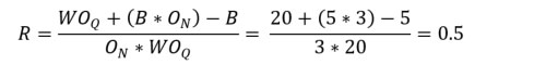
The Ratio R, equation 3, has a value of 0.5:

example 4

A simplistic visualization of the flow of batches through a WC on the right example 5
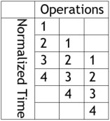
plots Operations on the horizontal with time on the vertical. The numbers symbolize the Batch number and their flow within the WC. The boxes symbolize all of the Standard Hours. Notice that if all the columns are shifted up to form a rectangle the Total Standard Hours formula becomes a simple area calculation.

The other key visualization here is the Flow Time. The height of the vertical axis is the Flow Time.

    The implications for the present system are that when serial lot-splitting is operational, this calculation is done for each applicable WO and WC, and the values of tWO1, n-1, tR,N, QN, YN, tR,N-1, and tQ,N-1 are adjusted accordingly.  References to Flow Time for a WO in this context refer to:

 equation 18

Adjusting for Parallel Lot-Splitting

When CN or CN-1 is greater than 0, WOs may be split and run through multiple paths in the WC.  This causes Flow Time to contract depending on the number of paths through which the WO is processed. When a lot is split when started, the present system first checks to validate the number of paths through which it is split versus the value of C in the WC, and then adjusts the Flow Time based on the ratio of the largest quantity sub-lot versus the # Units in the WO, RC.

equation 19

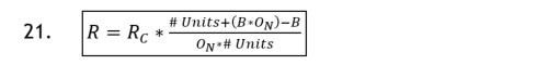
In this case, R can be further generalized as

equation 20

Or, from equation 16:

equation 21

Other Lot-Splitting Cases

There are other variations and combinations of lot-splitting cases that will also result in deviations between Flow Time and Standard Process Hours.  The derivations of these adjustments are not presented herein.

  • DCI Introduces Vortex Demand-Pull Technology +

    Since the early 1980's, the benefits of producing a given production volume throughput with the minimum amount of inventory have been well documented.  Beginning with the Just-in-Time methodologies, using Kanban cards for inventory replenishment, to Demand Flow methodologies,


    Read more
  • Vortex Introduction +

    The time-based demand-pull system (“demand-pull system”) technology of the described demand-pull system provides an implementation of demand-pull scheduling for various production operations/systems/factories.  It works in conjunction with a Material Resource Planning (MRP) or Enterprise Resource Planning (ERP) system, which creates production WOs and houses associated data, such as workflows and operational standard hours, to pull work through a factory with results similar to that of POLCA. 


    Read more
  • Production Priority-setting Examples +

        There are numerous methods of setting priorities in a production environment, too numerous to discuss in total in this paper, but some of the more prevalent methods are discussed below.


    Read more
  • First Authorized - First Processed Work Flow +

        When looking at work flow through a factory from the perspective of minimizing cycle time and honoring demand-pull policies, work should be processed on a first authorized, first processed (FAFP) basis. In other words, once a WO has been authorized within a WC’s queue, it should be pulled into production on a FAFP basis.  Deviating from this policy can result in an increase in the average cycle time, unless batching of WOs will reduce their aggregate cycle times due to machine capacity.  For an example of the latter situation, a machine may be capable of simultaneously processing ten pieces, and if there are two five-piece (or fewer) WOs, they could both be processed at the same time to reduce their aggregate cycle time, improve efficiency and maximize capacity.  


    Read more
  • Demand-Based Production from a Flow-Time Versus Need-Time Perspective +

    From a flow-time perspective, Work Orders should arrive in a Work Center's queue at precisely the time when they are needed to be worked on.  This minimizes both production cycle-time and inventory investment. The desired time for the next WO to arrive for processing is when the currently-authorized work in a WC and its upstream-adjacent (UA) WCs has been started into the WC and cleared the first operation in the WCs routing. This assumes that demand exists for the WO at the next downstream work cell.


    Read more
  • Examples of the Vortex Authorization Process +

    The examples set forth in the table below illustrate the WO authorization process resulting from the pull-test in different circumstances.  In all the examples, a set of WCs such as shown in the following Figure is used.  There are two WCs (WC 130 and WC 135) that feed into a third WC (WC 145) and the downstream WC (WC 145) is presumed to be healthy (reference the discussion of Work Center Performance Testing) so that the pull-testing for this WC is active. 


    Read more
  • Calculating Flow Time in a Work Center +

    Using Standard Labor/Machine Processing Hours
    In the case where all units in a WO are processed as a discrete set, the Flow Time of a WO in a WC is equal to the Standard Process Hours of the WO.


    Read more
  • Demand-Based Production from a Work-Volume Perspective +

    When looking at authorizing work in upstream stages of production, the traditional Kanban system establishes quantity buffers, or queues, at each WC. Then when the buffer quantity hits a minimum value (the Queue Policy), the Kanban card is returned to its originating WC for replenishment. 


    Read more
  • Table of Definitions +

    The following is a Table of Definitions for the articles describing the Vortex technology.


    Read more
  • An Optimum Queue Policy +
  • An Automated Demand-Pull System Embodiment +

    The Figures below illustrate an embodiment of the demand-pull system, which can be implemented using a software system with a database.  In this embodiment, a .NET service bus and MSSQL database running on a networked Microsoft Windows server are connected via the local area network (LAN) to individual clients in the various WCs. 


    Read more
  • Comparison of Time-Based Demand-Pull versus POLCA +

    POLCA (Paired Overlapping Loops of Cards with Authorization) is a prior art system to produce solutions to the application addressed herein, that is, demand-based shop floor control in a high mix, or high variety, production environment. 


    Read more
  • Vortex Shop Floor Control for Discrete Manufacturing +

    Is your manufacturing environment order-driven? Do you Engineer-to-Order or Customize-to-Order? Do your spaghetti diagrams look more like a network than continuous flow? If you struggle with production cycle-times that are too long and inventories that are too high, we have a solution!


    Introducing Vortex, a Shop Floor Control system designed to minimize your production cycle time and reduce inventory. Vortex works to pull production through your factory exactly when it’s needed! It predicts when a work center will be in need of more work, identifies the highest priority batch in all upstream work centers, and then authorizes the batch to be started just at the right time for it to reach the work center exactly when it is needed.


    Upstream work is only released if there is downstream demand, thus implementing one of the basic tenets of Lean Manufacturing – demand-pull production – in the high-variety, order-driven factory.


    Sounds simple, right?  In theory, yes.  However, if you’re talking dozens of work centers, dozens of different work flows and varying batches of sizes and flow times – predicting the time at which more work than is currently authorized for production will be needed can very quickly get complicated – the real-time calculations piling up pretty fast.

     
    Vortex streamlines the thousands of computations with a patent-pending algorithm, which works not only to synthesize all the math, but also integrate those solutions directly into your production system.


    Vortex’s modern, standards-based API is compatible with most ERP and Shop Floor Control systems.  The fully featured API allows your ERP and other internal systems to always stay up-to-date with the status of work on the shop floor. Vortex relies on your existing ERP system to create Work Orders according to your existing planning policies and inject them into the system through the API.  From there, Vortex handles the Starts into each work center based on demand-pull policies – minimizing both cycle-time and Work-in-Process inventories.  


    Check out our demo based on the following 5 products with individual work flows through 10 work centers. To view the demo, please click the link on this page - or drop us a line and we will take you for the tour.


    Read more